

Measuring Diversification Beyond Holdings and Average Correlations
Omaha, NE - September 2026
The Author
DyKa
Measuring Diversification Beyond Holdings and Average Correlation
Common risk structure, portfolio concentration, and losses in the tails
September 2026
Abstract
A portfolio can contain many investments without distributing risk across many distinct directions. Holdings count and average pairwise correlation describe useful features of a portfolio, but neither identifies its complete dependence structure or loss distribution. This paper separates three questions: how many positions are held, how return variation is distributed across statistical directions, and how portfolio losses behave in adverse states.
Two controlled experiments establish the distinction. First, twelve-asset portfolios with identical marginal volatilities and average correlations have the same equal-weight portfolio volatility, yet their correlation-matrix effective ranks are 7.26 and 3.93. Second, a Gaussian model and a two-state model are constructed with identical full covariance matrices. Their one-day 99% expected shortfalls are 1.81% and 2.68%, respectively. These are constructed examples, not forecasts or calibrated investment strategies.
An empirical illustration uses ten public U.S. industry portfolios over 2000-2025. Correlation-matrix effective rank is 3.46 over the full sample, 1.92 in 2008, and 1.62 in the first quarter of 2020. The 2022 experience is less uniform: volatility is higher than the full-sample estimate, while average correlation is slightly lower. Calendar subsamples and rolling estimates describe realized dependence; they do not establish causality or predictive power.
The contribution is a reproducible measurement framework, rather than a new diversification estimator. Read holdings count alongside correlation structure, portfolio-weighted risk contributions, and an explicit tail model. A lower effective rank indicates more concentrated statistical variation; it does not, by itself, establish a worse portfolio or a larger expected loss.
Scope
All empirical inputs are public research returns. All hypothetical parameters are disclosed. The analysis contains no private fund data, holdings, performance, or investment process. It does not estimate expected returns, optimize allocations, or evaluate an investable product. Figures, numerical outputs, and Python source accompany the paper.
1. What each measure can tell us
Portfolio variance depends on weights, individual volatilities, and pairwise relationships. This is the covariance-based starting point of portfolio analysis [1]. For a fully invested portfolio with weights w and covariance matrix Σ, variance is w′Σw. Write Σ = DCD, where D contains asset standard deviations and C is the correlation matrix.
A useful boundary condition
If all n assets have volatility σ and weight 1/n, the off-diagonal average correlation ρ̄ gives the exact identity:
σ²p = σ² [1/n + ((n − 1)/n)ρ̄].
Consequently, portfolios matched on these inputs cannot have different unconditional variances. Under zero-mean joint Gaussian returns, they also have the same portfolio loss distribution. A claim that hidden clusters alone increase their equal-weight Gaussian tail loss would contradict this identity. Once weights or individual volatilities differ, an unweighted average correlation no longer determines portfolio variance.
Count, dimension, and exposure
Holdings count measures the number of line items. Correlation-matrix effective rank measures the distribution of standardized return variation. Let λₖ be the nonnegative eigenvalues of C and define pₖ = λₖ / Σⱼλⱼ. Applying the entropy-based effective-rank definition of Roy and Vetterli [2] to C gives:
Neff(C) = exp[−Σₖ pₖ log(pₖ)], with 0 log(0) = 0.
For n uncorrelated assets, the measure is n; for perfectly identical standardized returns, it is one. Intermediate values describe spectral concentration, not a literal count of independent economic factors. Principal components are uncorrelated by construction, but need not be independent outside a Gaussian model. They also need not correspond to named economic exposures.
This statistic describes the asset universe, not the chosen allocation. It is invariant to rescaling individual returns before correlation is calculated. To describe the allocation, use the covariance matrix and the variance-contribution share:
RCᵢ = wᵢ(Σw)ᵢ / (w′Σw), with ΣᵢRCᵢ = 1.
These shares equal percentage contributions to volatility under the standard Euler decomposition. They can be negative for hedges. They identify which positions contribute to measured variance, while effective rank describes how broadly standardized variation is distributed. Neither is a substitute for an economic factor model or a tail-loss analysis.
2. Identical averages, different structures
Consider twelve hypothetical assets, each with zero mean and 1% daily volatility. Portfolio A assigns correlation 0.4121 to every distinct pair. Portfolio B has two clusters of eight and four assets, correlation 0.80 within each cluster, and zero correlation across clusters. There are 66 distinct pairs, of which 34 are within clusters; therefore B has average correlation 34 × 0.80 / 66 = 0.4121. Both matrices are positive definite.
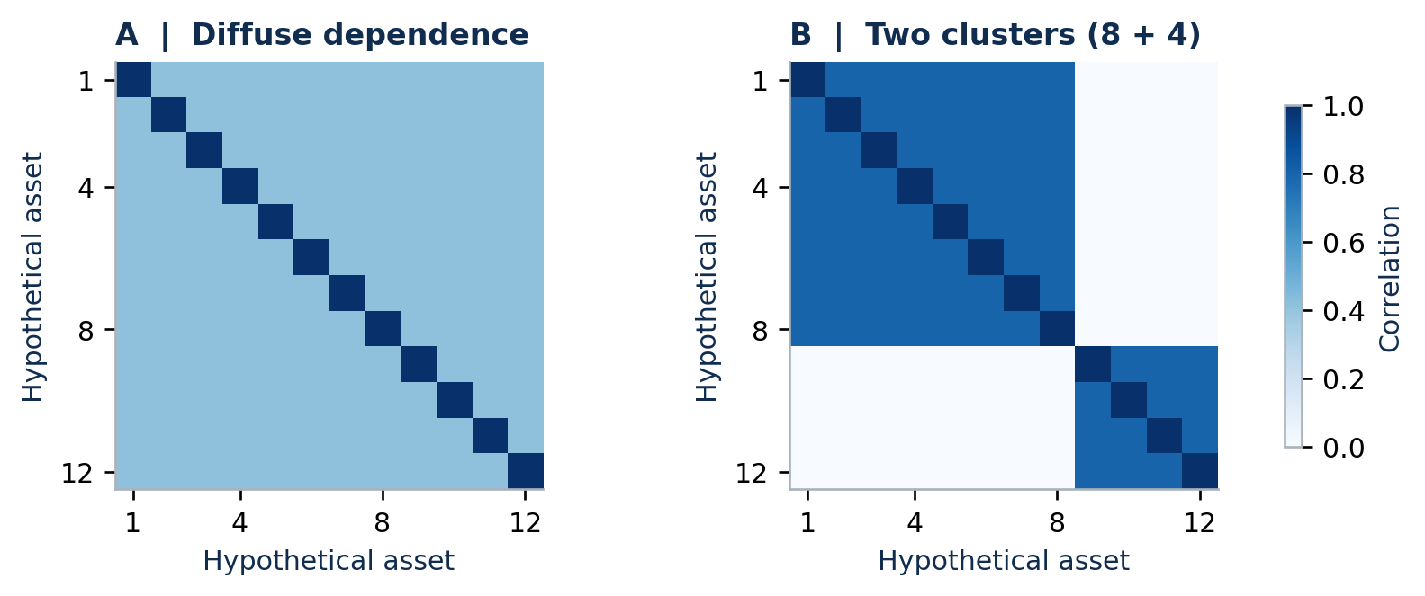
Figure 1. Constructed correlation matrices. Identical off-diagonal averages conceal different group structure. Asset labels are hypothetical; no market data enter this experiment.
| Measure | Diffuse (A) | Clustered (B) |
|---|---|---|
| Holdings / equal capital weights | 12 / 8.33% each | 12 / 8.33% each |
| Average correlation | 0.4121 | 0.4121 |
| Portfolio daily volatility | 0.679% | 0.679% |
| Correlation effective rank | 7.26 | 3.93 |
| First 8 assets: share of variance | 66.7% | 79.5% |
In B, each member of the larger cluster contributes 9.94% of portfolio variance; each member of the smaller cluster contributes 5.12%, despite identical capital weights and asset volatilities. The first eight assets contribute 79.5% of variance. In A, each asset contributes 8.33%. The same total risk can therefore be distributed differently across positions.
This matters when considering where to add capital or which group to shock. It does not establish that B has a worse equal-weight Gaussian loss distribution. A related limiting example is duplication: split each of three uncorrelated exposures into four identical positions and divide capital evenly. Holdings count rises from three to twelve, but portfolio returns are unchanged and correlation effective rank remains three.
3. Matching covariance does not match tails
The next experiment holds the entire unconditional covariance matrix fixed at A from Section 2. Model G is Gaussian. Model M is a zero-mean Gaussian mixture: 95% of observations use covariance Σ₀, while 5% use a high-volatility covariance 4Cₛ. Cₛ has diagonal one and off-diagonal correlation 0.90. Covariances are expressed in squared percentage-point units.
Σ₀ = (A − 0.05 × 4Cₛ) / 0.95; therefore E[Σstate] = A.
Σ₀ is positive definite. Its individual volatility is 0.918% and pairwise correlation 0.2902. In the rare state, individual volatility is 2%. Both unconditional models retain 1% individual volatility, correlation 0.4121, and equal-weight portfolio volatility 0.679%. State draws are independent over time; this is not a model of crisis duration.
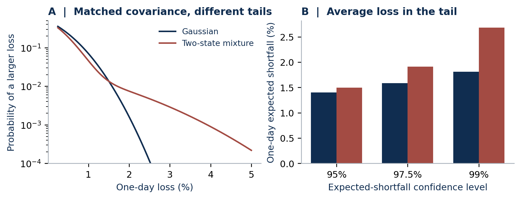
Figure 2. Analytical loss probabilities and expected shortfalls for the matched-covariance models. Daily loss units are percentage points. A 500,000-draw simulation per model independently checks the analytical results.
| One-day expected shortfall | Gaussian | Mixture | Difference |
|---|---|---|---|
| 95.0% | 1.40% | 1.49% | 6.6% higher |
| 97.5% | 1.59% | 1.91% | 20.3% higher |
| 99.0% | 1.81% | 2.68% | 48.3% higher |
Expected shortfall is the mean loss in the specified worst fraction of outcomes. At 99%, it averages the worst 1%. The larger difference deeper in the tail shows why the confidence level matters. Both models are symmetric: the rare state also produces large gains. The construction changes marginal tail thickness and state dependence together, so it does not isolate a pure correlation effect. It demonstrates that covariance alone does not identify tail losses.
4. Public-data illustration: ten industries
The empirical study uses daily value-weighted returns for ten U.S. industry portfolios from the Kenneth R. French Data Library [3]. Industries are formed using SIC classifications and reassigned annually. We use January 3, 2000 through December 31, 2025: 6,539 complete daily observations. Source percentage returns are divided by 100. The study uses total returns, not excess returns.
For portfolio calculations, each industry receives 10% weight each day, implying daily rebalancing across industry series before costs. This differs from the source’s value weighting within each industry. The ten portfolios are equity research series, not ten individual securities or a multi-asset opportunity set.
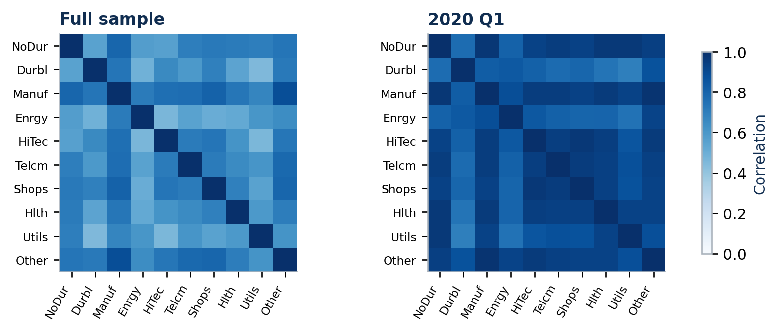
Figure 3. Public-data correlation estimates for the full sample and 2020 Q1. Labels follow the source file. Both panels use the same color scale. Source: Kenneth R. French Data Library; calculations in accompanying Python.
| Sample | Days | Avg. corr. | Eff. rank | Ann. vol. | Daily ES95 |
|---|---|---|---|---|---|
| Full sample | 6539 | 0.654 | 3.46 | 18.5% | 2.78% |
| 2008 | 253 | 0.844 | 1.92 | 39.0% | 6.07% |
| 2020 Q1 | 62 | 0.886 | 1.62 | 56.3% | 9.11% |
| 2022 | 251 | 0.647 | 3.24 | 22.6% | 3.17% |
Table 1. Volatility is daily sample standard deviation multiplied by √252, not a forecast. ES95 averages the worst ceil(0.05 × T) daily losses: 327, 13, 4, and 13 observations in the rows above. Short-sample tail estimates are especially unstable. Full sample includes all three event periods.
Industry count stays fixed while estimated dimension changes. In 2008 and early 2020, correlation is higher and effective rank lower than over the full sample. In 2022, volatility is elevated but average correlation is slightly lower. These selected, retrospective calendar comparisons illustrate different patterns; they do not imply that every stressed period produces a uniform rise in correlations.
5. Stability, sample size, and interpretation
Trailing 252-trading-day estimates show that statistical diversification varies within the same ten-industry universe. Each plotted point uses only observations through its ending date. However, no allocation rule is traded against these estimates, and the figure is not an out-of-sample forecasting test.
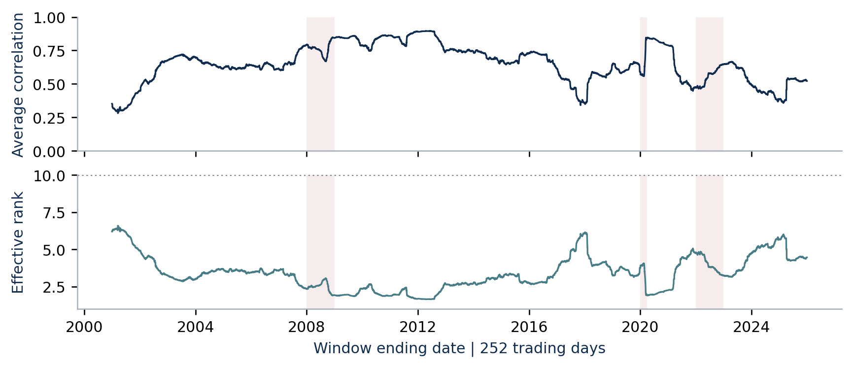
Figure 4. Rolling average correlation and correlation-matrix effective rank. Shading marks 2008, 2020 Q1, and 2022. Ten remains the maximum possible effective rank. Overlapping windows create mechanically smooth, dependent estimates.
| Sample | Effective rank | Bootstrap 95% range |
|---|---|---|
| Full sample | 3.46 | 3.09 to 3.87 |
| 2008 | 1.92 | 1.64 to 2.54 |
| 2020 Q1 | 1.62 | 1.45 to 3.35 |
| 2022 | 3.24 | 2.83 to 3.62 |
Table 2. Percentile ranges from 500 circular moving-block bootstrap samples with 20-trading-day blocks; all ten return columns are resampled together. These are conditional resampling ranges, not calibrated forecasts or formal tests of differences across nested samples.
The early-2020 sample yields a wide range, not a precise count of surviving diversifiers. Block resampling preserves local runs but cannot reproduce absent crises. Within-period stationarity is a strong approximation, and effective-rank estimates have finite-sample bias.
As a lookback sensitivity check, estimates sampled every 21 trading days have median effective ranks of 3.25, 3.30, and 3.19 for 126-, 252-, and 504-day windows. This broad agreement concerns typical levels, not identical turning points. Shorter windows react faster and contain less information.
Extreme-return conditioning can itself alter correlations; Longin and Solnik [4] explain why a suitable null model matters. Calendar windows avoid selecting individual returns by magnitude, but differences in volatility, composition, and sample size remain. This is descriptive evidence.
6. A practical reading of diversification
The experiments support a layered interpretation. An average correlation can summarize total equal-weight variance under restrictive conditions while concealing the location of risk. A complete covariance matrix can identify variance while leaving substantial uncertainty about tail losses. The empirical results show why these distinctions should be revisited across windows rather than collapsed into a permanent diversification label.
Begin with the economic exposure
Count positions, but examine whether they respond to shared drivers. An industry label, legal wrapper, or additional line item does not establish a new return source. The duplication example is deliberately extreme; in practice, partial overlap requires judgment about economic sensitivity alongside return-based evidence. This study does not identify causal drivers from principal components.
Read structure together with capital allocation
Inspect the correlation matrix and its spectrum, then calculate risk contributions using actual weights and volatilities. Correlation effective rank is intentionally weight-free. A portfolio can have access to many statistical directions while allocating almost all risk to one. Conversely, a low-dimensional universe can contain a useful hedge if its exposures are combined appropriately. Maximizing effective rank is therefore not an investment objective on its own.
State what the stress assumption changes
Stress analysis should identify whether it changes individual volatilities, correlations, expected returns, liquidity, or several at once. Experiment 2 specifies both higher volatility and stronger common dependence in a rare state and offsets them in the normal state to preserve unconditional covariance. Its larger expected shortfall cannot be attributed to correlation alone. Undisclosed assumptions would make an apparently precise stress result difficult to interpret.
Separate descriptive evidence from a forecast
Historical estimates describe the observations used to construct them. A prospective decision requires an independently specified rule, a training period, an evaluation period, and treatment of trading costs and estimation error. None is supplied here because the question is measurement, not investment performance. The chosen event windows are illustrations rather than an exhaustive catalog of difficult markets.
Limitations and conclusion
The empirical universe contains U.S. equities only. Results cannot establish how credit, rates, commodities, currencies, derivatives, or illiquid assets diversify one another. Pearson correlation measures linear dependence; it does not capture every nonlinear relationship. The simulations omit serial clustering, transaction costs, liquidity constraints, and asymmetric shocks. Historical datasets can be revised, and bootstrap ranges do not remove model risk.
Within these limits, the conclusion is precise: position count, dependence structure, and tail exposure answer different questions. Use them together. More holdings do not necessarily create new statistical dimensions, and matching variance does not necessarily match downside outcomes. Neither observation invalidates diversification; both improve the specificity with which it can be measured.
Appendix. Reproduction and references
Computational specification
The companion reproduce.py downloads the source archive only when no local copy exists, reads the first daily value-weighted block, filters the stated date range, checks for missing sentinel values and duplicate dates, and writes decimal returns plus derived outputs. It uses the July 2026 CRSP-based source vintage retrieved September 7, 2026. The archive checksum is recorded in results.json; the packaged copy fixes the inputs used here. Later source revisions may change results.
Correlation is Pearson sample correlation. Eigenvalues are obtained by a symmetric eigensolver; tiny negative numerical values are clipped to zero, and zero entropy terms are omitted. No shrinkage is applied. The correlation-matrix spectrum is used throughout: applying effective rank to a return matrix or covariance matrix would answer a different question. Volatility uses sample standard deviation with one degree-of-freedom correction.
For the tail experiment, loss L is measured in percentage points. Let Φ and φ be the standard normal distribution and density. The Gaussian loss standard deviation is 0.67905. The mixture standard deviations are 0.54236 and 1.90613 with probabilities 0.95 and 0.05. Solve Σⱼπⱼ[1 − Φ(q/sⱼ)] = α for q; then ES = Σⱼπⱼsⱼφ(q/sⱼ) / α. All reported model ES values are analytical. Simulation projects each state directly to the equal-weight portfolio, which is distributionally equivalent to drawing the multivariate model and then applying the weights.
Monte Carlo uses NumPy seed 20260907 and 500,000 observations per model. Bootstrap uses seed 1701, 500 replicates, and circular blocks of length 20; indices wrap within each sample and excess draws are truncated. Sensitivity calculations advance by 21 observations from the first eligible endpoint for each lookback, so their endpoint grids differ. The code checks covariance matching, positive definiteness, and Monte Carlo agreement with analytical results.
References
[1] Markowitz, H. (1952). Portfolio Selection. The Journal of Finance, 7(1), 77-91. Source.
[2] Roy, O., and Vetterli, M. (2007). The Effective Rank: A Measure of Effective Dimensionality. EUSIPCO, 606-610. Source.
[3] French, K. R. Data Library: 10 Industry Portfolios, daily returns and construction details. Accessed September 7, 2026. Source.
[4] Longin, F., and Solnik, B. (2001). Extreme Correlation of International Equity Markets. The Journal of Finance, 56(2), 649-676. Source.
Research use
This paper is educational research, not a recommendation, forecast, or representation of any fund. Hypothetical results are not realized investment performance. Public research portfolios do not represent returns available to an investor after trading costs. No affiliation with the cited authors or data provider is implied.
Disclaimer
The information provided in this article is for informational and educational purposes only. DyKa Investments, LLC does not provide personalized investment advice, and nothing in this article constitutes financial, investment, legal, or other professional advice. Readers should not interpret this content as an endorsement of any specific investment strategy, asset, or financial instrument.
This article does not take into account the specific investment objectives, financial situation, or individual needs of any particular person. It should not be relied upon as the sole basis for making any investment decisions. Readers are encouraged to conduct their own research and consult with a licensed financial advisor before making any investment decisions.
Additionally, this material may not be reproduced, distributed, or used in any manner without the prior written consent of DyKa Investments, LLC. Unauthorized use or reproduction of this content is strictly prohibited and may be subject to legal action.
DyKa Investments, LLC expressly disclaims any and all liability in respect of actions taken or not taken based on any or all of the contents of this article.